Metric-Based Few-Shot Learning

Metric-based approaches to few-shot learning are able to learn an embedding space where examples that belong to the same class are close together according to some metric, even if the examples belong to classes that were not seen during training.

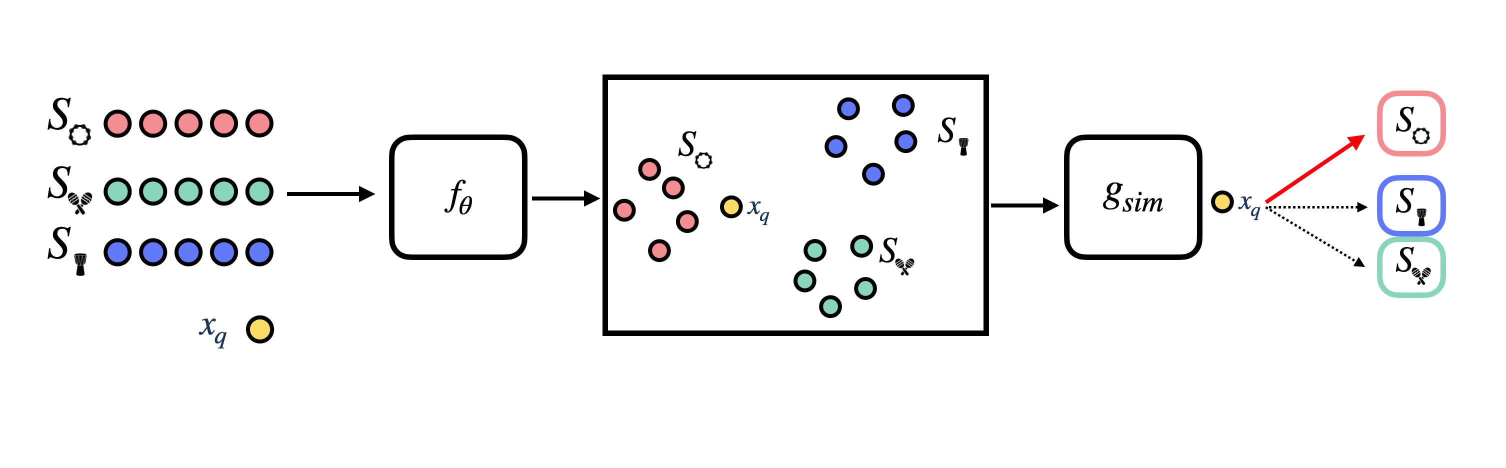
At the center of metric-based few-shot learning approches is a similarity metric, which we will refer to as \(g_{sim}\). We use this similarity metric to compare how similar examples in the query set are to examples in the support set. After knowing how similar a query example is to each example in the support set, we can infer to which class in the support set the query example belongs to. Note that this is conceptually the same as performing a nearest neighbor search.

This similarity comparison is typically done in the embedding space of some neural net model, which we will refer to as \(f_\theta\). Thus, during episodic training, we train \(f_\theta\) to learn an embedding space where examples that belong to the same class are close together, and examples that belong to different classes are far apart. This embedding model is sometimes also referred to as a backbone model.

There are many different metric-based approaches to few-shot learning, and they all differ in how they define the similarity metric \(g_{sim}\), and how they use it to compare query examples to support examples as well as formulate a training objective.

Among the most popular metric-based approaches are Prototypical Networks [16], Matching Networks [14], and Relation Networks [17].

Example: Prototypical networks

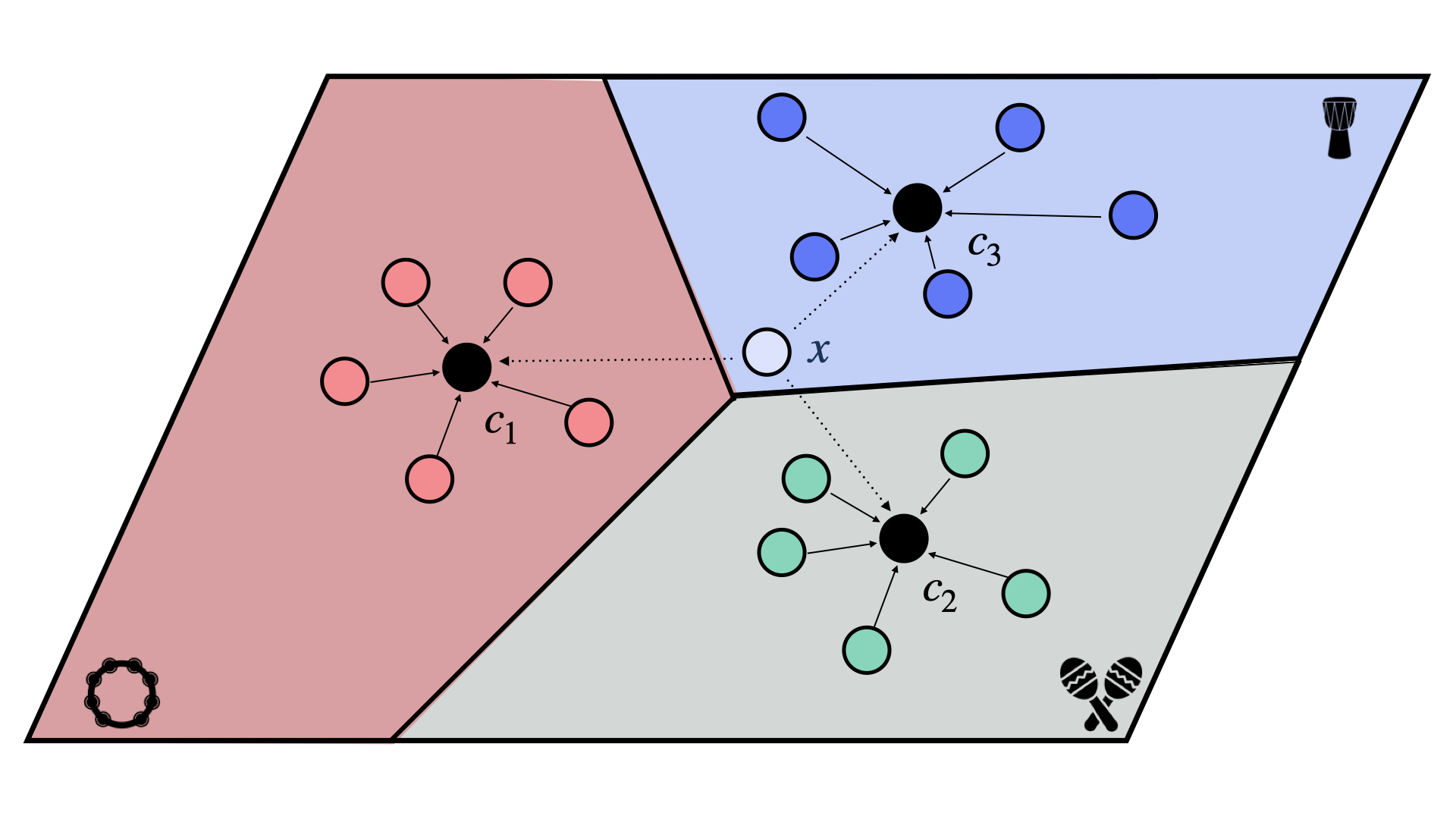
Fig. 4 The figure above illustrates a 5-shot, 3-way classification task between tambourine (red), maracas (green), and djembe (blue). In prototypical networks, each of the 5 support vectors are averaged to create a prototype for each class (\(c_k\)). The query vector \(x\) is compared against each of the prototypes using squared eucldean distance. The query vector (shown as \(x\)) is assigned to the class of the prototype that it is most similar to. Here, the prototypes \(c_k\) are shown as black circles.

Prorotypical networks [16] work by creating a single embedding vector for each class in the support set, called the prototype. The prototype for a class is the mean of the embeddings of all the examples in the support set for that class.

The prototype (denoted as \(c_k\)) for a class \(k\) is defined as:

\[ c_k = 1 / |S_k| \sum_{x_k \in S_k} f_\theta(x_k) \]

where \(S_k\) is the set of all examples in the support set that belong to class \(k\), \(x_k\) is an example in \(S_k\), and \(f_\theta\) is the backbone model we are trying to learn.

After creating a prototype for each class in the support set, we use the euclidean distance between the query example and each prototype to determine which class the query example belongs to. We can build a probability distribution over the classes by applying a softmax function to the negated distances between a given query example and each prototype:

\[ p(y = k | x_q) = \frac{exp(-d(x_q, c_k))}{\sum_{k'} exp(-d(x_q, c_{k'}))} \]

where \(x_q\) is a query example, \(c_k\) is the prototype for class \(k\), and \(d\) is the squared euclidean distance between two vectors.

Prototypical Networks are Zero-Shot Learners too!

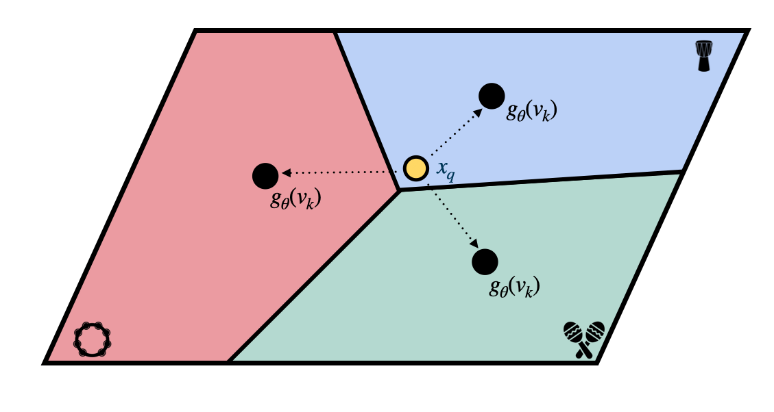
Fig. 5 When used for zero-shot learning (ZSL), prototypical networks don’t require a labeled support set of examples for each class. Instead, the model is trained using a set of class metadata vectors, which are vectors that describe the characteristics of each class that the model should be able to classify. These metadata vectors are mapped to the same embedding space as the inputs using a separate model, \(g_\theta\), and used as the prototypes for each class. The prototypical network then uses the distances between the input and the class prototypes to make predictions about the input’s category.

The prototypical network method can also be used for zero-shot learning. The method remains mostly the same as above. However, instead of relying on a support set \(S_k\) for each class \(k\), we are given some class metadata vector \(v_k\) for each class.

The class metadata vector \(v_k\) is a vector that contains some information about the class \(k\), which could be in the form of a text description of the class, an image, or any other form of data. During training, we learn a mapping \(g_\theta\) from the class metadata vector \(v_k\) to the prototype vector \(c_k\): \(c_k = g_\theta(v_k)\).

In this zero-shot learning scenario, we are mapping from two different domains: the domain of the class metadata vectors \(v_k\) (ex: text) and the domain of the query examples \(x_q\) (ex: audio). This means that we are learning two different backbone models that map to the same embedding space: \(f_\theta\) for the input query and \(g_\theta\) for the class metadata vectors.

For more information on zero-shot learning, see the Zero-Shot Learning section.