Zero-Shot Learning Foundations

Zero-shot learning (ZSL) is yet another approach for classifying the classes that are not observed during training. Main difference from few-shot learning is that it does not require any additional label data for novel class inputs.

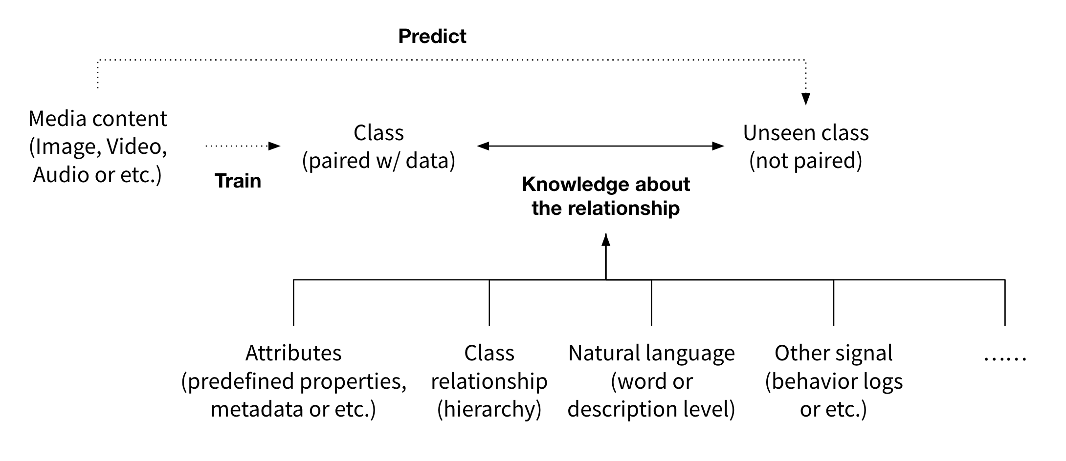
Therefore, in zero-shot learning, there is no further training step for unseen classes. Instead, during the training phase, the model learns how to use the side information that can potentially cover the relationship between any of both seen and unseen classes. After training, it can handle the cases where inputs from unseen classes are to be classified.

ZSL was originally inspired by human’s ability to infer novel objects or create new categories dynamically based on prior semantic knowledge, where general relationship between seen and unseen classes are learned.

Overview on Zero-shot Learning Paradigm

Let’s look into a case of an audio-based instrument classication task. First, given training audio and their associated class labels (seen classes), we train a classifier that projects input vectors onto the audio embedding space.

However, there isn’t a way to make prediction of unseen labels for unseen audio inputs yet.

As forementioned we use the side information that can inform the relationships between both seen and unseen labels. There are various sources of the side information, such as class-attribute vectors infered from an annotated dataset, or general word embedding vectors trained on a large corpus of documents. We will go over in detail in the later section.

The core of zero-shot learning paradigm is to learn the compatibility function between the embedding space of the inputs and the side information space of their labels.

• Compatibility function : \(F(x, y ; W)=\theta(x)^T W \phi(y)\)

  • \(\theta(x)\) : input embedding function.

  • \(W\) : mapping function.

  • \(\phi(y)\) : label embedding function.

A typical approach is to train a mapping function between the two. By unveiling relationship between the side information space and the our input feature space, it is possible to map vectors from one space to the other.

After training, arbitrary inputs of unseen labels can be predicted to the corresponding class.

Another option is to train a separate zero-shot embedding space where the embeddings from both spaces are projected (a metric-learning approach).

• E.g. Training mapping functions \(W_1\) and \(W_2\) with a pairwise loss function : \(\sum_{y \in \mathcal{Y}^{seen}}\left[\Delta\left(y_n, y\right)+F\left(x_n, y ; W_1, W_2\right)-F\left(x_n, y_n ; W_1, W_2\right)\right]_{+}\)

  • where \(F(x, y ; W_1, W_2)= -\text{Distance}(\theta(x)^T W_1, \phi(y)^T W_2)\)

In this case, the inputs and the classes are projected onto another zero-shot embedding space.

This space-aligning technique is one of the main branches of zero-shot learning framework. Next, we’ll go over another branch or research direction, the generative approach.

One example of the generative approach is to employ a conditional Generative Adversarial Network (GAN) to generate samples related to the unseen classes. Its training process is consist of two parts.

At the first part of the training phase, with the audio data annotated with the seen classes, we train the GAN architecture (a generator and a discriminator) combined with the audio encoder and an additional classification model. The convolutional neural network (CNN) audio encoder will try to embed the audio into the CNN feature vectors that well represents the class characteristics by being evaluated by the discriminator. At the same time, given the class representative vectors we get from the side information space, the generator will try to mimic the CNN audio feature vector that is produced by the audio encoder. There could be an additional classification module that is aimed to classify the labels from the generated CNN audio feature vector. This module helps the regularization of the GAN framework.

After training the GAN framework, we can now generate the CNN audio feature vector of an arbitrary unseen class, given the class’ representative vector on the side information space.

With the help of the generative model, we can actually generate as many vector samples we want for a certain class.

After generating a sufficient number of the CNN audio feature vector, we now have a paired dataset (CNN audio feature vector / their labels) for training a classifier for the unseen classes. This is the second part of the training phase.

We could also train a classifier in the generalized zero-shot evaluation manner.

After training, we are now ready with the audio encoder and the classifier. The model can make prediction of unseen classes given the audio input.

So far, we’ve gone through the broad concepts of the two major zero-shot learning paradigms. Next, we’ll look more into the detailed task formulation.