Optimization-Based Few-Shot Learning

Optimization-based approaches focus on learning model parameters \(\theta\) that can easily adapt to new tasks, and thus new classes. The canonical method for optimization-based few-shot learning is Model-Agnostic Meta Learning (MAML) [18], and it’s successors [19, 20].

The intuition behind MAML is that some representations are more easily transferrable to new tasks than others.

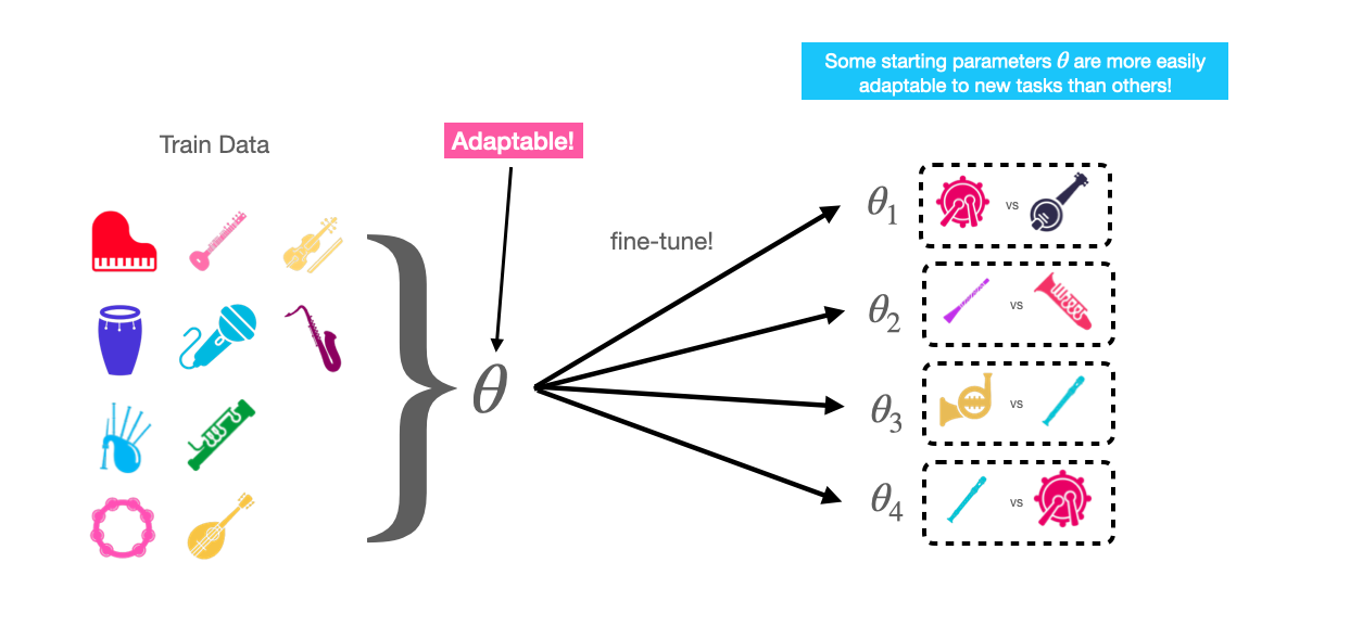
For example, assume we train a model with parameters \(\theta\) to classify between (piano, guitar, saxophone and bagpipe) samples. Normally, we would expect that these parameters \(\theta\) would not be useful for classifying between instruments outside the training distribution, like cello and flute. The goal of MAML is to be able to learn parameters \(\theta\) that are useful not just for classifying between the instruments in the training set, but also are easy to adapt to new instrument classification tasks given a support set for each task, like cello vs flute, violin vs trumpet, etc.

In other words, if we have some model parameters \(\theta\), we want \(\theta\) to be adapted to new tasks using only a few labeled examples (a single support set) in a few gradient steps.

The MAML algorithm accomplishes this by training the model to adapt from a starting set of parameters \(\theta\) to a new set of parameters \(\theta_i\) that are useful for a particular episode \(E_i\). This is performed for all episodes in a batch, eventually learning a starting set of parameters \(\theta\) that can be successfully adapted to new tasks using only a few labeled examples.

Note that MAML makes no assumption of the model architecture, thus the “model-agnostic” part of the method.

The MAML algorithm

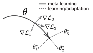
Fig. 6 The MAML algorithm [18]. The starting model parameters are depcted as \(\theta\), while the task-specific, fine-tuned parameters for tasks 1, 2, and 3 are depicted as \(\theta_1^*\), \(\theta_2^*\), and \(\theta_3^*\), respectively.

Suppose we are given a meta-training set composed of many few-shot episodes \(D_{train} = \{E_1, E_2, ..., E_n\}\), where each episode contains a support set and train set \(E_i = (S_i, Q_i)\). We can follow the MAML algorithm to learn parameters \(\theta\) that can be adapted to new tasks using only a few examples and a few gradient steps.

Overview of the MAML algorithm [18]:

1. Initialize model parameters \(\theta\) randomly, choose a step sizes \(\alpha\) and \(\beta\).

2. while not converged do

   1. Sample a batch of episodes (tasks) from the training set \(D_{train} = \{E_1, E_2, ..., E_n\}\)

   2. for each episode \(E_i\) in the batch do

      1. Using the current parameters \(\theta\), compute the gradient of the loss \(L_if(\theta)\) for episode \(E_i\).

      2. Compute a new set of parameters \(\theta_i\) by fine-tuning in the direction of the gradient w.r.t. the starting parameters \(\theta\): \(\theta_i = \theta - \alpha \nabla_{\theta} L_i\)

   3. Using the fine-tuned parameters \(\theta_i\) for each episode, make a prediction and compute the loss \(L_{i}f(\theta_i)\).

   4. Update the starting parameters \(\theta\) by taking a gradient step in the direction of the loss we computed with the fine-tuned parameters \(L_{i}f(\theta_i)\):

      \(\theta = \theta - \beta \nabla_{\theta} \sum_{E_i \in D_{train}}L_i f(\theta_i)\)

At inference time, we are given a few-shot learning task with support and query set \(E_{test} = (S_{test}, Q_{test})\). We can use the learned parameters \(\theta\) as a starting point, and follow a process similar to the one above to make a prediction for the query set \(Q_{test}\):

1. Initialize model parameters \(\theta\) to the learned parameters from meta-training.

2. Compute the gradient \(\nabla_{\theta} L_{test} f(\theta)\) of the loss \(L_{test}f(\theta)\) for the test episode \(E_{test}\).

3. Similar to step 6 of the training algorithm above, compute a new set of parameters \(\theta_{test}\) by fine-tuning in the direction of the gradient w.r.t. the starting parameters \(\theta\).

4. Make a prediction using the fine-tuned parameters \(\theta_{test}\): \(\hat{y} =(\theta_{test})\).