Evaluating (and Visualizing) a Trained Prototypical Net#

We’ve made it to the last part of this coding tutorial, hooray!

In this section, we’ll evaluate our trained prototypical network on the our unseen musical instrument classes, and visualize the embedding space for the entire evaluation dataset, as well as individual episodes.

Requirements (hidden)

%%capture
!pip install "torchmetrics==0.10.2" 
!pip install torch
!pip install tqdm
!pip install numpy
!pip install --no-cache-dir --upgrade music-fsl

from pathlib import Path

import numpy as np
import torch
import tqdm
from torchmetrics import Accuracy

from music_fsl.protonet import PrototypicalNet
from music_fsl.backbone import Backbone
from music_fsl.train import FewShotLearner, TEST_INSTRUMENTS
from music_fsl.util import dim_reduce, embedding_plot, batch_device
from music_fsl.data import TinySOL, EpisodeDataset

Loading from Checkpoint#

The first thing we will do is load our trained model from checkpoint.

%%capture
# download a checkpoint from the repo (for colab compatibility)
!wget https://github.com/music-fsl-zsl/music_fsl/raw/main/checkpoints/epoch%3D0-step%3D600.ckpt

checkpoint_path = "epoch=0-step=600.ckpt"
DEVICE = "cuda" if torch.cuda.is_available() else "cpu"
sample_rate = 16000

protonet = PrototypicalNet(Backbone(sample_rate))
learner = FewShotLearner.load_from_checkpoint(checkpoint_path, protonet=protonet)
learner.eval()
learner = learner.to(DEVICE)

Instantiating our Test Data#

Now, we can load a set of test episodes to evaluate on. We’ll evaluate our model on the same 5-way, 5-shot paradigm that we used to train. Again, we’ll use the EpisodeDataset class to create our test episodes.

n_way = 5
n_support = 5
n_query = 15
n_episodes = 50 

# load our evaluation data
test_episodes = EpisodeDataset(
    dataset=TinySOL(
        instruments=TEST_INSTRUMENTS, 
        sample_rate=sample_rate
    ), 
    n_way=n_way, 
    n_support=n_support,
    n_query=n_query, 
    n_episodes=n_episodes
)

INFO: Downloading ['audio', 'annotations'] to /home/hugo/mir_datasets/tinysol
INFO: [audio] downloading TinySOL.tar.gz
INFO: /home/hugo/mir_datasets/tinysol/audio/TinySOL.tar.gz already exists and will not be downloaded. Rerun with force_overwrite=True to delete this file and force the download.
INFO: [annotations] downloading TinySOL_metadata.csv
INFO: /home/hugo/mir_datasets/tinysol/annotation/TinySOL_metadata.csv already exists and will not be downloaded. Rerun with force_overwrite=True to delete this file and force the download.

Setting up our Metrics#

To keep things simple, we’ll simply compute the per-episode accuracy for our model. Using the average=samples parameter in the Accuracy metric, we can compute the accuracy for each episode, and then average the accuracies over all episodes.

# instantiate the accuracy metric
metric = Accuracy(num_classes=n_way, average="samples")

The Evaluation Loop#

We’ll do two things main things in our evaluation loop:

Compute the accuracy for each episode, and average over all episodes.
Collect an embedding table with support, query, and prototype embeddings for each episode. We’ll use this embedding table later to visualize the embedding space for each episode. We’ll store the embedding table in a list of dictionaries, where each dictionary contains one embedding, with it’s corresponding label, type (i.e. support, query, or prototype), and episode number.

# collect all the embeddings in the test set
# so we can plot them later
embedding_table = []
pbar = tqdm.tqdm(range(len(test_episodes)))
for episode_idx in pbar:
    support, query = test_episodes[episode_idx]

    # move all tensors to cuda if necessary
    batch_device(support, DEVICE)
    batch_device(query, DEVICE)

    # get the embeddings
    logits = learner.protonet(support, query)

    # compute the accuracy
    acc = metric(logits, query["target"])
    pbar.set_description(f"Episode {episode_idx} // Accuracy: {acc.item():.2f}")

    # add all the support and query embeddings to our records
    for subset_idx, subset in enumerate((support, query)):
        for emb, label in zip(subset["embeddings"], subset["target"]):
            embedding_table.append({
                "embedding": emb.detach().cpu().numpy(),
                "label": support["classlist"][label],
                "marker": ("support", "query")[subset_idx], 
                "episode_idx": episode_idx
            })
        
    # also add the prototype embeddings to our records
    for class_idx, emb in enumerate(support["prototypes"]):
        embedding_table.append({
            "embedding": emb.detach().cpu().numpy(),
            "label": support["classlist"][class_idx],
            "marker": "prototype", 
            "episode_idx": episode_idx
        })

Episode 49 // Accuracy: 0.81: 100%|██████████| 50/50 [03:34<00:00,  4.29s/it]

Sweet! Now that we’ve iterated through all of our test episodes, we can compute the average accuracy for our model by calling metric.compute()

# compute the total accuracy across all episodes
total_acc = metric.compute()
print(f"Total accuracy, averaged across all episodes: {total_acc:.2f}")

Total accuracy, averaged across all episodes: 0.75

Visualizing the Embedding Space#

We can visualize the embedding space for the entire dataset, as well as for each episode. We’ll make use of two helper functions: dim_reduce for performing dimensionality reduction to 2 or 3 dimensions on our embedding table, and embedding_plot for plotting the reduced embeddings.

def dim_reduce(
        embeddings: np.ndarray, 
        n_components: int = 3,
        method: str= 'umap',
    ):
    """
    This function performs dimensionality reduction on a given set of embeddings. 
    It can use either UMAP, t-SNE, or PCA for this purpose. The number of components 
    to reduce the data to and the method used for reduction can be specified as arguments. 
    It returns the projected embeddings as a NumPy array.

    Args:
        embeddings (np.ndarray): An array of embeddings, with shape (n_samples, n_features)
        n_components (int): The number of dimensions to reduce the embeddings to. Default: 3
        method (str): The method of dimensionality reduction to use.
                        One of 'umap', 'tsne', or 'pca'. Default: 'umap'

    Returns:
        proj (np.ndarray): The dimensionality-reduced embeddings, with shape (n_samples, n_components)
    """

def embedding_plot(
        proj: np.ndarray, 
        color_labels: List[Union[int, str]], 
        marker_labels: List[int] = None,
        title: str = ''
    ):
    """
    Plot a set of embeddings that have been reduced using dim_reduce.

    Args:
        proj: a numpy array of shape (n_samples, n_components)
        color_labels: a list of labels to color the points by
        marker_labels: a list of labels to use as markers
        title: the title of the plot

    Returns:
        a plotly figure object
    """

Although the details of the implementation of these two functions are beyond the scope of this tutorial, you can look at the implementation in the util.py file of this tutorial’s accompanying repo.

# perform a TSNE over all embeddings in the test dataset
embeddings = dim_reduce(
    embeddings=np.stack([d["embedding"] for d in embedding_table]),
    method="tsne",
    n_components=2,
)

# replace the original 512-dim embeddings with the 2-dim tsne embeddings
# in our embedding table
for entry, dim_reduced_embedding in zip(embedding_table, embeddings):
    entry["embedding"] = dim_reduced_embedding

/home/hugo/conda/envs/hugo/lib/python3.8/site-packages/sklearn/manifold/_t_sne.py:996: FutureWarning: The PCA initialization in TSNE will change to have the standard deviation of PC1 equal to 1e-4 in 1.2. This will ensure better convergence.
  warnings.warn(

Now that we have our dim-reduced embeddings in our embedding table, we can go ahead and plot a TSNE embedding of the entire dataset.

fig = embedding_plot(
    proj=np.stack([d["embedding"] for d in embedding_table]),
    color_labels=[d["label"] for d in embedding_table],
    marker_labels=[d["marker"] for d in embedding_table],
    title="TinySOL Protonet Embeddings",
)

fig.show()

Looks like our model learned a decent discriminative embedding spcae for our unseen musical instrument classes!

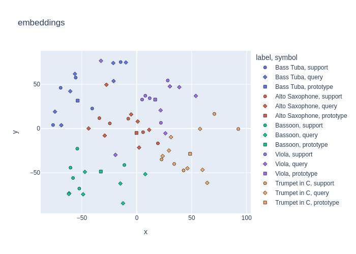
To take a closer look at what happens during a few-shot learning episode, we can plot the embedding space only for a single episode.

episode_idx = 5

subtable = [d for d in embedding_table if d["episode_idx"] == episode_idx]

fig = embedding_plot(
    proj=np.stack([d["embedding"] for d in subtable]),
    color_labels=[d["label"] for d in subtable],
    marker_labels=[d["marker"] for d in subtable],
    title=f"episode {episode_idx} -- embeddings",
)
fig.show()

Few-shot and Zero-shot Learning for Music Information Retrieval

Evaluating (and Visualizing) a Trained Prototypical Net

Contents